In this handbook, I introduce and discuss key corporate finance concepts. The framework is intended to give a broad overview, as well as some specifics for each topic, to aid people working on building models for FP&A and related operations. While it is primarily geared toward developers, it also serves to help the finance subject matter experts understand the bridge terminology between finance and technology.
Gaining a general understanding of basic Finance and Accounting concepts as well as Financial Statement Analysis will increase the usefulness and relevance of the models we build. And Finance teams will appreciate the modeling examples, as it helps them learn the language of the modeling components.
The focus of this document is on teaching the common financial concepts we run into every day building TM1 models. (Note that IBM Planning Analytics is referred to as “TM1” for short in this document.)
This is not a best practices document for TM1 development.
The examples given in the "TM1 Modeling tips" are meant to be illustrative and help the developer bridge the finance knowledge to TM1. Since the goal is to “connect the dots” between finance concepts and TM1 modeling concepts, only a few examples are provided, and they are generally the simpler examples. My goal is to build a bridge for communication here, not write the final word on TM1 architecture.
If you have TM1 examples that you think would be helpful to include, please email Robin Stevens rstevens@cubewise.com
There are many factors that contribute to architecting a multi-dimensional model, it’s not a “one approach suits all” situation. Factors for great model architecture (which is beyond the scope of this document) and determining best practices include:
• Size of data set
• Number of users
• Complexity of calculations
• Use cases for model (reporting? Journal entries?)
• Interplay between model being designed and other models/systems
In addition, my experience is primarily with U.S. based companies and their policies. Most accounting practices internationally are similar to the U.S. GAAP standards, although there are differences. And, worldwide, all companies track expenses, capital, people, products/services, although approaches may vary.
Lastly, I wanted to mention that although the examples within are for IBM Planning Analytics (aka TM1), many of the same concepts of how to model finances apply regardless of the software utilized. So, my hope is that this guide is useful to developers and finance teams across the world.
The Chart of Accounts (CoA) is the structural foundation of any financial model, including those built in IBM Planning Analytics (TM1). It lists every account used in the client’s financial system, mapping each account to a financial statement (either the Balance Sheet or the Income Statement) and to a logical section within that statement (e.g., Cash & Equivalents, Accounts Receivable, Inventory, etc.).
Here is a sample of a Chart of Accounts:
Account | Fin Statement | Section |
|---|---|---|
11115 - SVB Sweep | BS | Cash & Equiv |
11121 - WFB CC - USD | BS | Cash & Equiv |
11122 - WFB CC - UK | BS | Cash & Equiv |
11123 - WFB - USD | BS | Cash & Equiv |
11125 - WFB - EUR | BS | Cash & Equiv |
11145 - Cash Clearing | BS | Cash & Equiv |
11210 - Short-term Investment | BS | Cash & Equiv |
12010 - Accounts Receivable Trade | BS | Accounts Receivable |
12025 - Unbilled Receivable | BS | Accounts Receivable |
12070 - Allowance for Doubtful Accounts | BS | Accounts Receivable |
12120 - Intercompany Interest Receivable | BS | Accounts Receivable |
12190 - Intercompany Receivables | BS | Accounts Receivable |
14010 - Raw Material | BS | Inventory |
14013 - Raw Material-Preapproval | BS | Inventory |
14020 - Work in Process - Material | BS | Inventory |
14030 - Work in Process - Material Overhead | BS | Inventory |
14070 - Sub-Assembly | BS | Inventory |
14080 - Finished Goods | BS | Inventory |
14090 - Accruals and Adjustments | BS | Inventory |
Accounting Fundamentals
COA table | |
|---|---|
1XXX | Assets |
2XXX | Liabilities |
3XXX | Equity |
4XXX | Revenue |
5XXX | COGS |
6XXX | Operating Expense |
7XXX | Interest |
8XXX | Taxes |
9XXX | Other Non-Operating Expense |
TM1 Modelling Tips
The Trial Balance is a core input into any TM1 model that deals with FP&A data. It represents the financial state of a company at a point in time and includes the activity and balances of all accounts—both income statement and balance sheet. It’s often delivered monthly and may be segmented by other fields such as department or legal entity.
This report is usually structured with one row per account and columns for various balance types (e.g., beginning balance, activity, ending balance, debits, credits). It reflects the debits and credits for each account and follows fundamental accounting rules that must be understood when importing into TM1:
Debits & Credits
Here is a sample showing the first few rows of a Trial Balance:
Account | Beg Bal | Debit | Credit | Activity | End Bal |
|---|---|---|---|---|---|
11115 - SVB Sweep | (2,224,804) | 638,627,166 | 639,066,628 | 439,462 | (2,664,266) |
11121 - WFB CC - USD | 8,580,780 | 292,967,055 | 293,042,221 | 75,165 | 8,505,615 |
11122 - WFB CC - UK | 5,376,223 | 45,050,977 | 40,755,386 | (4,295,591) | 9,671,815 |
11123 - WFB - USD | 821,747 | 815,804 | 1,035,881 | 220,077 | 601,670 |
11125 - WFB - EUR | 196,080 | 1,332,885 | 1,167,920 | (164,964) | 361,045 |
11145 - Cash Clearing | 2,206,141 | 21,188,619 | 17,781,726 | (3,406,893) | 5,613,034 |
11210 - Short-term Investment | 1,663,207 | 10,507,931 | 11,889,108 | 1,381,177 | 282,030 |
12010 - Accounts Receivable Trade | 477,603 | 4,894,219 | 5,246,815 | 352,595 | 125,007 |
12025 - Unbilled Receivable | 152,939 | 231,345 | 275,963 | 44,618 | 108,320 |
TM1 Modeling Tips
The Income Statement (IS), also commonly referred to as the P&L (Profit & Loss) is the financial report that shows how much money a company earned and spent during a given period—typically a month, quarter, or year. In TM1 and most FP&A models, the values for the income statement represent the “activity” for that period (as described in previous sections.)
Of all financial statements, the income statement is the most scrutinized—especially in a corporate planning context—because it directly reflects profitability and business performance.
Accounting Fundamentals
TM1 Modeling Tips
TM1 Modeling Tips
A Cash Flow Statement consists of 3 areas:
TM1 Modeling Tips
Sample Cash Flow Structure showing data sources
Cash Flow Section | Line Item Description | Input/Rule Driven | Notes/Source |
|---|---|---|---|
Starting Cash | Ending cash from prior period | Rule-driven | Based on previous period |
Operating Activities | |||
Net Income | Rule-driven | From IS | |
Stock-Based Compensation | Rule-driven | From IS – non-cash | |
Depreciation & Amortization | Rule-driven | From IS – non-cash | |
Change in Prepaids and Current Assets | Rule-driven | Delta from BS | |
Change in Other Assets | Rule-driven | Delta from BS | |
Change in Accounts Payable | Rule-driven | Delta from BS | |
Change in Accrued Liabilities | Rule-driven | Delta from BS | |
Change in Other Liabilities | Rule-driven | Delta from BS | |
Change in Cash – Operating | Calculated | Sum of above | |
Investing Activities | |||
CapEx | Rule-driven | From CapEx model | |
Purchase of Investments | Input | Often for M&A | |
Maturity of Investments | Input | Often for M&A | |
Change in Cash – Investing | Calculated | Sum of above | |
Financing Activities | |||
Equity Issuance / Buybacks | Input | Stock issuance/repurchases | |
Debt Increase / Repayment | Input | Loans, bonds, etc. | |
Dividends Paid | Input | Cash dividends | |
Change in Cash – Financing | Calculated | Sum of above | |
Ending Cash | Sum of net change in cash + starting cash | Roll-up | Output metric |
The Income Statement and the Balance Sheet carry all the day to day transactions for a given company, and allow us to review trends, analyze performance, and better understand the workings of an organization.
While much attention is paid to profit margins, which are calculated based on Income Statement data only, key ratios are often comprised of data that comes from both the Income Statement and the Balance Sheet. These ratios are helpful in summarizing large amounts of financial data spread across multiple reports, and include things like ROA (Return on Assets), Inventory Turnover, and Accounts Receivable Days. See Common Key Performance Indicators for more on this topic.
Both statements provide most of the information needed to derive a Cash Flow statement as well. The diagram below shows the sources for different key parts of the Cash Flow statement.
Interplay Between Statements
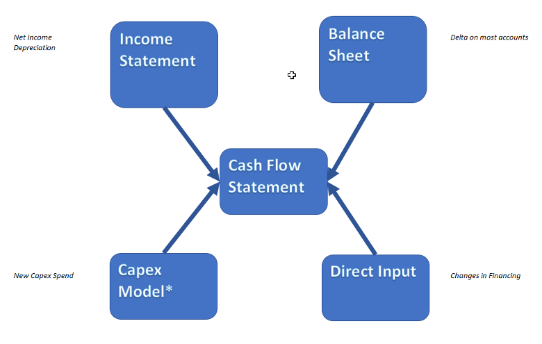
Statement | Notes |
|---|---|
Income Statement | Key drivers: Net Income, Depreciation (non-cash items) |
Balance Sheet | Monthly deltas (Δ) used to calculate operating cash flows |
Capex Model | Capex spend typically drives investing activities |
Direct Inputs | Used for Financing: Debt, Equity, Dividends |
TM1 Modeling Tips
Definition & Formula
Booking Timing
General Ledger Behavior
IS → BS Link
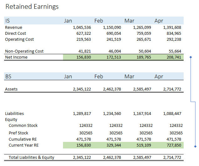
Retained Earnings links together the results from any given year of the Income Statement to the Balance Sheet. Basically, Net Income is deemed to be value generated by the company. They can either pay out the proceeds in dividends (which has become much less common over time as companies favor growth) or reinvest the money in the company, at which point it becomes equity.
Example:
Currency Note (for Multicurrency TM1 Models)
TM1 Modeling Tips
Expense Allocations are a common calculation for both Actual and Forecast data for most companies. While Direct Costs are generally easily matched to the revenues they produce, a large portion of expenses are spread across the activities of the entire organization. These costs are Operating Costs.
When measuring the success of a business, it is helpful to allocate a portion of these Operating Costs to different products/regions/business activities to get a better sense of overall profitability. Gross Margin will tell us the contribution made after making and selling products, but the activities of marketing, offices, management, IT, and more are not taken into account in Gross Margin.
Allocations often cause a significant amount of angst amongst department managers, as it is very hard to agree on an allocation methodology that feels “fair” to all. But they are a useful analytical tool, and as such, it’s best to keep allocation methods as simple as possible, and avoid the temptation to make too many exceptions to your general allocation rubric.
Generally, operating costs are allocated based on another metric such as Revenue, Expense, Headcount, or Square Footage. Here are some common examples:
Discussing allocations can get confusing, so it’s best to agree on some terminology when trying to understand a company’s allocation methodology. Here is a helpful rubric:
The Rubric | Description | Example |
|---|---|---|
Source | What dollars are being allocated | Most common: Facilities & IT Depts |
Target | Where are dollars being allocated | Generally all Departments except the Source Depts |
Basis | How are dollars spread | Same as Target (make sure denominator does not include Source Depts) Usually Headcount or Total Expense |
Contra | Where do contra dollars go | Most common: Facilities & IT Depts |
Sequence | What order do allocations occur? | Additional level of complexity. Requires multiple additional rollups of Depts/Accounts Only necessary when one allocation is dependent on another |
TM1 Modeling Tips
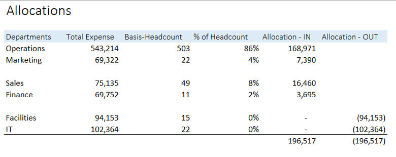
The example below shows Facilities and IT expenses being allocated to the other departments in the organization, using Headcount as a Basis:
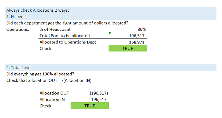
When testing allocations, use these two methods:
KPI stands for Key Performance Indicator. It is a broadly used term that can refer to any metric—ratios, percentages, dollar values, or units—that helps assess business performance.
KPIs are used to:
There are many industry-specific KPIs, but most planning models include a set of common corporate finance KPIs. These should be clearly defined, consistently calculated, and easily explainable to stakeholders.
Common KPIs in Corporate Planning Models
The table below describes some of the most common KPIs, and their purpose.
**Profitability ** | |
|---|---|
Gross Margin % Operating Margin % | Direct from IS, measures profit contributed less direct production costs Direct from IS, measures profit contributed less operating costs |
Net Margin % | Direct from IS, measures profit contributed less taxes and financing ("bottom line") |
** Liquidity ** | |
EBIT | EBIT = Earnings Before Interest & Taxes. Similar to Operating Profit (difference is usually "extraordinary items" associated with one-time investments or acquisitions.) Indicator of earnings generated prior to financing considerations. |
EBITDA | EBITDA =Earnings Before Interest, Taxes, Depreciation, and Amortization. Proxy for "operating cash flow", as it excludes the largest non-cash transactions (depreciation), as well as removing financing related accounts. Popular as a short-cut to Cash Flow. |
Working Capital | Current Assets - Current Liabilities. Measure of liquidity, shows your "cash" (or near-cash) position. Helpful especially for start-ups or fast growing companies that are funding growth directly. Indicates ability to meet (or not) short term obligations. If it is negative, company is at risk of missing payments. |
AR Days | AR Days (Accounts Receivable Days) = the number of days that a customer invoice is outstanding before it is collected. This is relevant for credit sales (non-cash) Also called as Debtor Days or DSO (Days Sales Outstanding) |
AP Days | AP Days (Accounts Payable Days) = the number of days it takes to clear all outstanding Accounts Payable. This concept is useful for determining how efficient the company is at clearing whatever short-term account obligations it may have Also called as Creditor Days or DPO (Days Payable Outstanding) |
** Asset Management ** | |
Inventory Days | Inventory days = the number of days it takes for inventory to turn into sales Also called as Inventory Outstanding |
Asset Turnover | Asset turnover = Total Sales or Revenue / Average Assets This metric helps investors understand how effectively companies are using their assets to generate sales. Investors use the asset turnover ratio to compare similar companies in the same sector or group |
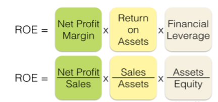
The importance of Financial Statement analysis can be summarized by reviewing the set of KPIs known as “Dupont Analysis”, which is shown below. Basically, it breaks apart a typical ROE equation into a profit component and an asset component. By reviewing the pieces of ROE, you can determine if a company is good at managing costs, and/or good at managing assets. This breakdown also makes comparisons to competitors more meaningful.
TM1 Modeling Tips
Revenue recognition is one of the most foundational accounting principles in corporate finance. It determines when and how a company recognizes revenue on its financial statements. Under accrual accounting, revenue is recognized when it is earned and realized—not necessarily when the cash is received.
This becomes especially important in situations like long-term contracts, subscription services, or multi-year software licenses.
Accounting Fundamentals
Sales vs. Revenue
Though sometimes used interchangeably, Sales and Revenue are distinct:
Sales Forecasting
Sales forecasting is the estimation of future revenue, based on historical trends, current pipeline data, and industry conditions. It’s a critical input to revenue planning models.
Common Forecasting Inputs:
Methods Include:
The method selected will depend on:
TM1 Modeling Tips
Capital Expenditures (Capex) refer to the funds used by a company to acquire, upgrade, and maintain physical assets such as property, buildings, or equipment. These are long-term investments that are capitalized on the balance sheet and depreciated over time rather than being expensed immediately.
Capex differs from operational expenses (Opex), which are short-term costs incurred in the day-to-day functioning of the business. Capex decisions are often tied to strategic initiatives like growth, capacity expansion, or digital transformation.
Depreciation, which is expensed each month, can be thought of as the cost of using a particular asset for that time. While there are many methods of depreciation, a simple straight-line depreciation is the most common. This simply takes the asset value divided by the asset life. For example, new cubicles would be considered “leasehold improvements” and might be depreciated over 10 years. So, $1m invested in new cubicles would be recorded on the Balance Sheet, and $100,000 per year would be funnelled through the Income Statement as an expense (and deprecate the investment on the Balance Sheet by the same amount.)
Accounting Treatment:
TM1 Modeling Tips
General Info
Seasonality refers to the predictable, recurring changes in business activity that occur generally within a one-year period. These fluctuations are driven by calendar events, commercial cycles, or environmental factors such as weather. Understanding and modeling seasonality is essential for accurate forecasting, especially for companies whose demand or spending patterns vary significantly throughout the year.
Examples:
Seasonality can affect not just Revenue, but also Expenses, Headcount, Cash Flow, and even Capex timing. Correctly modeling it helps ensure that forecasted results align with operational realities.
Approaches to Calculating Seasonality
Approach 1: Mechanical (TM1 Rules-Based)
This is the most common method used in financial planning systems when prior-year data is available.
This approach uses simple proportional logic to spread forecasted annual revenue across months based on historical patterns. It works well when the company’s seasonality is stable year-over-year.
Approach 2: AI-Driven (Advanced Forecasting)
For more complex or volatile businesses, an AI-based approach can produce more refined seasonal forecasts.
This method is particularly valuable when external data (e.g., weather, promotions, or macroeconomic indicators) influences performance.
TM1 Modeling Tips
FP&A Overview
Employee benefits represent the non-salary compensation that companies provide to employees, including bonuses, insurance, retirement contributions, and other employment-related costs.
In financial planning, benefits are often modeled as a combination of percentages of salary and fixed costs per employee (FTE). Accurate modeling helps ensure total personnel expense forecasts are realistic and aligned with company policies and statutory requirements.
Common Benefit Types and Calculation Methods
Timing Considerations
TM1 Modeling Tips
Building employee benefit calculations in TM1 (Planning Analytics) should balance accuracy and model simplicity.
FP&A Overview
A Bill of Materials (BOM) lists every component, material, and sub-assembly required to produce a finished good. It is central to operational finance and manufacturing planning because it drives both inventory management and cost calculation.
For example, a car’s BOM might include thousands of parts—everything from the cloth for the seats and the plastic for the dashboard to the screws that hold everything together. Managing this complexity efficiently helps balance production capacity, cash flow, and inventory costs.
Key considerations include:
Efficient management of these factors allows for just-in-time inventory, minimal waste, and optimal cash utilization—all key outcomes for FP&A teams monitoring working capital and cost of goods sold (COGS).
Because BOMs are hierarchical (e.g., the car seat has its own sub-BOM for covers, foam, and metal), financial models may need to summarize or “roll up” costs across multiple levels of the hierarchy.
TM1 Modeling Tips
In TM1 or other planning systems, BOMs can be modeled at varying levels of detail depending on the use case:
When done well, a TM1 BOM model can connect operational manufacturing data to the financial forecast, providing valuable insights into COGS, cash flow, and margin performance.
Accounting Overview
Standard costing is a cornerstone of manufacturing accounting and works hand-in-hand with the Bill of Materials (BOM). It allows businesses to assign consistent, pre-determined costs to products, making budgeting, forecasting, and variance analysis more efficient.
Each period (typically annually), companies set standard costs for each component of production based on historical data, supplier pricing, and operational expectations. These standards are used to calculate the Cost of Goods Sold (COGS) and are applied to the actual number of units produced.
Standard costs are usually divided into three categories:
As production occurs, actual costs are tracked and compared against these standards. The differences—variances—are analyzed to understand operational performance and cost control effectiveness. Variances are recorded in both the Income Statement (COGS section) and the Balance Sheet (Inventory accounts).
Typical variances include:
TM1 Modeling Tips
In most systems, the ERP handles actual costing (including variances), while TM1 handles forecasting and planning. The modeling objective is to make standards flexible and responsive to volume or price changes.
Key modeling tips:
This approach ensures the forecasting model mirrors operational realities while remaining easy to adjust and maintain.
Key FX Rates
Model Types
Type | Description |
|---|---|
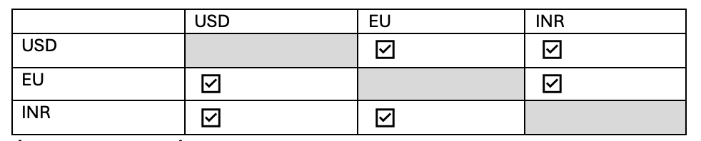
Multi-Currency Model | Translates every currency to every other currency. Rare; used when many intercompany transactions occur across global entities. |
Reporting Currency Model | Most common; translates all local currencies to a single parent reporting currency (e.g., everything → USD). |
Examples:
Multi-currency matrix:
Reporting-currency mapping:
Local Currency | Reporting Currency |
|---|---|
USD | USD |
EU | USD |
INR | USD |
Constant Currency
Constant Currency is used in FP&A to isolate true operational performance by removing the impact of foreign exchange (FX) rate movements. Instead of translating results using current-period FX rates, all periods are translated using a fixed reference rate (often prior year actuals, prior forecast, or a defined budget rate).
From a business perspective, constant currency allows finance and business partners to separate out variances caused by business activities (higher sales, deferred expenses, etc.) from those caused by currency fluctuations.
TM1 Modeling Tips
Intercompany transactions occur between two entities within the same parent company. They must be eliminated during consolidation so internal activity doesn’t distort revenue, expenses, assets, or liabilities.
Common intercompany scenarios:
Actuals vs Forecast
TM1 Modeling Tips
Example:
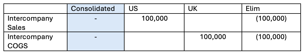
Result: No internal revenue or expense remains at consolidation.
4. GL Account Structure
Billings, bookings, and backlog are closely related but distinct metrics that help FP&A track revenue, sales performance, and future business obligations. Understanding their differences is key for accurate forecasting and financial modeling.
Metric | Timing Focus | Purpose | Example Focus |
|---|---|---|---|
Bookings | Contract signing | Measure sales success & demand | Total value of signed contracts in a month |
Billings | Invoice issuance | Track cash flow & collections | Monthly invoices sent to customers |
Backlog | Future delivery | Forecast revenue/workload | Value of signed contracts yet to be fulfilled |
Definitions and Examples
Key Relationship:
Backlog = Bookings – Billings
TM1 Modeling Tips
Acronym | Definition | Where used |
|---|---|---|
COA | Chart of Accounts | Financial Statements |
AP | Accounts Payable | Balance Sheet |
AR | Accounts Receivable | Balance Sheet |
BS | Balance Sheet | Financial Statements |
CF | Cash Flow | Financial Statements |
CIP | Capital Investment Project | Alternate name for Capex (used mostly by non-profits and government) |
COGS | Cost of Goods Sold | Income Statement |
CR | Credit | Trial Balance |
DR | Debit | Trial Balance |
EBIT | Earnings Before Income & Taxes | Financial Analysis |
EBITDA | Earnings Before Income, Taxes, Depreciation, and Amortization | Financial Analysis |
F&F | Furniture & Fixtures | Capex |
Fx | Exchange Rates | Assumptions |
G&A | General & Administrative | Income Statement |
GM | Gross Margin | Income Statement |
IS | Income Statement | Financial Statements |
ITD | Inception to Date | Financial Statements |
KPI | Key Performance Indicator | Financial Statements |
NI | Net Income | Financial Statements (also called Net Profit and sometimes Net Margin) |
P&L | Profit & Loss | Financial Statements - synonym for IS |
PP&E | Property, Plant & Equipment | Balance Sheet |
QTD | Quarter to Date | Financial Statements |
R&D | Research & Development | Income Statement |
SG&A | Sales, General & Administrative | Income Statement |
YTD | Year to Date | Financial Statements |
Common Terms | Definition |
|---|---|
Matching Principal | This is the concept that companies must book all revenue and expense for a certain activity in the same period. It is to ensure that companies do not over/understate their income. |
Accruals | At the end of a month, companies must book any expenses that are associated with that month, even if they have not yet paid the expenses. These are "accruals". They get booked to the Balance Sheet, generally as a Current Asset. The following month, when the item is paid for, it is expensed (on the Income Statement), and the accrual for the prior month is reversed (a negative mirror amount is entered in the current month) |
Debits & Credits | Debits and credits are equal but opposite entries in your books. If a debit increases an account, you will decrease the opposite account with a credit. A debit is an entry made on the left side of an account. It either increases an asset or expense account or decreases equity, liability, or revenue accounts. |
Activity & Balance | The difference between the Debit and Credit on an account for a single time period (such as a month or a year) is called the account's "activity" for that period. "Activity" is used in IS and CF. The "balance" is the ending balance for the same period in question. The ending balance is an accumulation of ALL activity (since the company's inception) on a single account. "Balances" are used in Capital planning and the BS. |
Double-entry bookkeeping | This is the basis for all modern accounting. It means, when you record a transaction, it is always entered in two different places. For example, when you make a sale, it is recorded as Revenue, and also as Cash. The double-entry system ensures all accounts are integrated and balance out. |
Controllable Expenses | This is a subset of Operating Expense, which only includes those expenses that a Manager has some control over. It includes employee related expenses, travel, consultants but excludes things like depreciation, allocations, or acquisition costs. This is to allow for managers to be measured only by that which they control. |
Drivers | Drivers are generally quantities that influence an expense item. For example, a driver for rent expense is number of employees, since that drives how much space is needed. A "driver-based model" is one where users input the drivers (such as square footage, market share, number of employees), and the expenses are then calculated. |
Allocation | Generally used to indicate expenses that are booked to one department, but the cost must be shared with other departments. Expenses are usually allocated based on Headcount, although other metrics (Total Expense, Square Footage, % of Sales, etc.) may also be used. |
Fund Accounting | An alternative accounting setup used by Government & Non-profits. Difference is it focuses on matching funds and costs, which is equivalent to revenue and costs. |